LPrec
Here is an example on how to use the log-polar based method (https://github.com/math-vrn/lprec) for reconstruction in Tomopy
%pylab inline
Install lprec from github, then
import tomopy
DXchange is installed with tomopy to provide support for tomographic data loading. Various data format from all major synchrotron facilities are supported.
import dxchange
matplotlib provide plotting of the result in this notebook. Paraview or other tools are available for more sophisticated 3D rendering.
import matplotlib.pyplot as plt
Set the path to the micro-CT data to reconstruct.
fname = '../../tomopy/data/tooth.h5'
Select the sinogram range to reconstruct.
start = 0
end = 2
This data set file format follows the APS beamline 2-BM and 32-ID definition. Other file format readers are available at DXchange.
proj, flat, dark, theta = dxchange.read_aps_32id(fname, sino=(start, end))
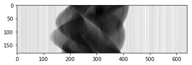
Plot the sinogram:
plt.imshow(proj[:, 0, :], cmap='Greys_r')
plt.show()
If the angular information is not avaialable from the raw data you need to set the data collection angles. In this case theta is set as equally spaced between 0-180 degrees.
theta = tomopy.angles(proj.shape[0])
Perform the flat-field correction of raw data:
proj = tomopy.normalize(proj, flat, dark)
Select the rotation center manually
rot_center = 296
Calculate
proj = tomopy.minus_log(proj)
proj[proj<0] = 0
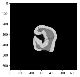
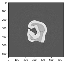
Reconstruction using FBP method with the log-polar coordinates
recon = tomopy.recon(proj, theta, center=rot_center, algorithm=tomopy.lprec, lpmethod='fbp', filter_name='parzen')
recon = tomopy.circ_mask(recon, axis=0, ratio=0.95)
plt.imshow(recon[0, :,:], cmap='Greys_r')
plt.show()
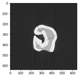
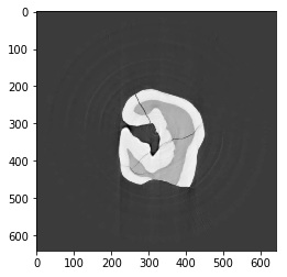
Reconstruction using the gradient descent method with the log-polar coordinates
recon = tomopy.recon(proj, theta, center=rot_center, algorithm=tomopy.lprec, lpmethod='grad', ncore=1, num_iter=64, reg_par=-1)
recon = tomopy.circ_mask(recon, axis=0, ratio=0.95)
plt.imshow(recon[0, :,:], cmap='Greys_r')
plt.show()
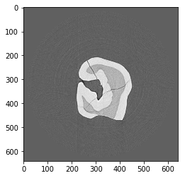
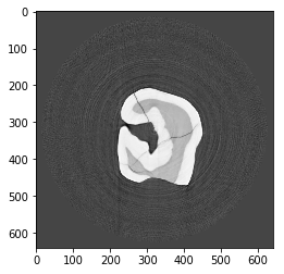
Reconstruction using the conjugate gradient method with the log-polar coordinates
recon = tomopy.recon(proj, theta, center=rot_center, algorithm=tomopy.lprec, lpmethod='cg', ncore=1, num_iter=16, reg_par=-1)
recon = tomopy.circ_mask(recon, axis=0, ratio=0.95)
plt.imshow(recon[0, :,:], cmap='Greys_r')
plt.show()
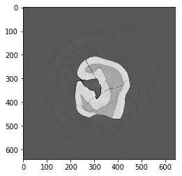
Reconstruction using the TV method with the log-polar coordinates. It gives piecewise constant reconstructions and can be used for denoising.
recon = tomopy.recon(proj, theta, center=rot_center, algorithm=tomopy.lprec, lpmethod='tv', ncore=1, num_iter=512, reg_par=5e-4)
recon = tomopy.circ_mask(recon, axis=0, ratio=0.95)
plt.imshow(recon[0, :,:], cmap='Greys_r')
plt.show()
Reconstruction using the TV-entropy method with the log-polar coordinates. It can be used for suppressing Poisson noise.
recon = tomopy.recon(proj, theta, center=rot_center, algorithm=tomopy.lprec, lpmethod='tve', ncore=1, num_iter=512, reg_par=2e-4)
recon = tomopy.circ_mask(recon, axis=0, ratio=0.95)
plt.imshow(recon[0, :,:], cmap='Greys_r')
plt.show()
Reconstruction using the TV-l1 method with the log-polar coordinates. It can be used to remove structures of an image of a certain scale, and the regularization parameter \(\lambda\) can be used for scale selection.
recon = tomopy.recon(proj, theta, center=rot_center, algorithm=tomopy.lprec, lpmethod='tvl1', ncore=1, num_iter=512, reg_par=3e-2)
recon = tomopy.circ_mask(recon, axis=0, ratio=0.95)
plt.imshow(recon[0, :,:], cmap='Greys_r')
plt.show()
Reconstruction using the MLEM method with the log-polar coordinates
recon = tomopy.recon(proj, theta, center=rot_center, algorithm=tomopy.lprec, lpmethod='em', ncore=1, num_iter=64, reg_par=0.05)
recon = tomopy.circ_mask(recon, axis=0, ratio=0.95)
plt.imshow(recon[0, :,:], cmap='Greys_r')
plt.show()