Vector Reconstruction
The vector reconstruction algorithm can be used for instance, to reconstruct the magnetization vector field inside a magnetic sample.
Here is an example on how to use the vector reconstruction algorithm [B6] [A3] with TomoPy[A1].
From a reconstructed 3D object to its projections and back
In order to test the algorithm, the projections of a reconstructed oject can be computed, and from these projections we can come back to the reconstructed model object. Finally we will compare the results of the vector field reconstruction against the initial object.
All datasets used in this tutorial are available in tomoBank.
First, let’s make the necessary imports
import dxchange
import tomopy
import numpy as np
import matplotlib.pyplot as plt
import time
Let’s load the object: the three components of the magnetization vector all throughout the object. The object will be padded in order to have a cubic object. Afterwards it will be downsampled to make faster computations.
obx = dxchange.read_tiff('M4R1_mx.tif').astype('float32')
oby = dxchange.read_tiff('M4R1_my.tif').astype('float32')
obz = dxchange.read_tiff('M4R1_mz.tif').astype('float32')


npad = ((182, 182), (64, 64), (0, 0))
obx = np.pad(obx, npad, mode='constant', constant_values=0)
oby = np.pad(oby, npad, mode='constant', constant_values=0)
obz = np.pad(obz, npad, mode='constant', constant_values=0)

obx = tomopy.downsample(obx, level=2, axis=0)
obx = tomopy.downsample(obx, level=2, axis=1)
obx = tomopy.downsample(obx, level=2, axis=2)

oby = tomopy.downsample(oby, level=2, axis=0)
oby = tomopy.downsample(oby, level=2, axis=1)
oby = tomopy.downsample(oby, level=2, axis=2)

obz = tomopy.downsample(obz, level=2, axis=0)
obz = tomopy.downsample(obz, level=2, axis=1)
obz = tomopy.downsample(obz, level=2, axis=2)
Define the projection angles: 31 angles, from 90 to 270 degrees:
ang = tomopy.angles(31, 90, 270)
And calculate the projections of the object taking rotation axes around the three perpendicular cartesian axes:
prj1 = tomopy.project3(obx, oby, obz, ang, axis=0, pad=False)
prj2 = tomopy.project3(obx, oby, obz, ang, axis=1, pad=False)
prj3 = tomopy.project3(obx, oby, obz, ang, axis=2, pad=False)
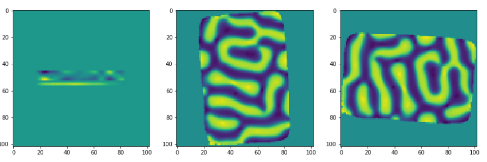
The three coordinates of a given projection can be visualized as follows:
fig = plt.figure(figsize=(15, 8))
ax1 = fig.add_subplot(1, 3, 1)
ax1.imshow(obx[52,:,:])
ax2 = fig.add_subplot(1, 3, 2)
ax2.imshow(oby[52,:,:])
ax3 = fig.add_subplot(1, 3, 3)
ax3.imshow(obz[52,:,:])
Finally we will reconstruct the vector field components, taking as input the projections that we have calculated thanks to the first 3D initial object. The number of iterations can be adapted to have a faster but more imprecise reconstruction, or to have a more precise reconstruction.
rec1, rec2, rec3 = tomopy.vector3(prj1, prj2, prj3, ang, ang, ang, axis1=0, axis2=1, axis3=2, num_iter=100)
dxchange.write_tiff(rec1)
dxchange.write_tiff(rec2)
dxchange.write_tiff(rec3)
Comparison of results against input object
In this section, we compare the results of the vector field components obtained thanks to the tomopy reconstruction, against the vector field components of the object given as input:
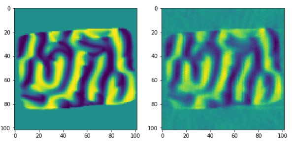
Comparison of the first magnetization vector component against the input data object (for a given slice).
fig = plt.figure(figsize=(9, 7))
ax1 = fig.add_subplot(1, 2, 1)
ax1.imshow(obx[52,:,:])
ax2 = fig.add_subplot(1, 2, 2)
ax2.imshow(rec1[52,:,:])
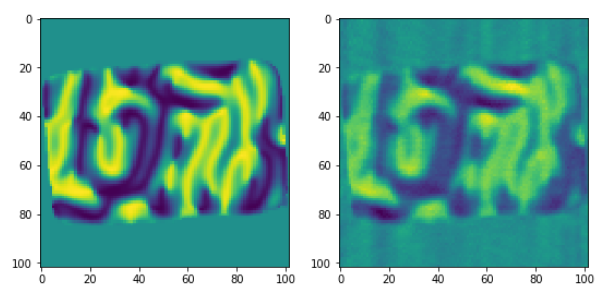
Comparison of the second magnetization vector component against the input data object (for a given slice):
fig = plt.figure(figsize=(9, 7))
ax1 = fig.add_subplot(1, 2, 1)
ax1.imshow(oby[52,:,:])
ax2 = fig.add_subplot(1, 2, 2)
ax2.imshow(rec2[52,:,:])
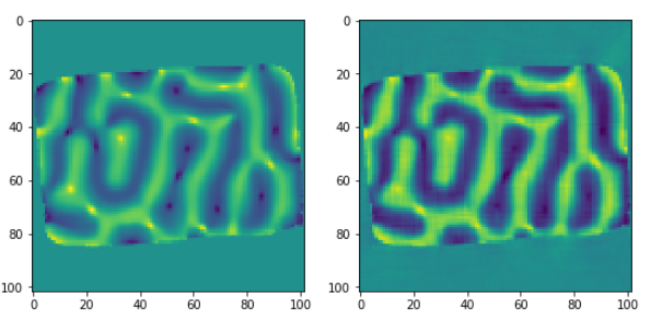
Comparison of the third magnetization vector component against the input data object (for a given slice):
fig = plt.figure(figsize=(9, 7))
ax1 = fig.add_subplot(1, 2, 1)
ax1.imshow(obz[52,:,:])
ax2 = fig.add_subplot(1, 2, 2)
ax2.imshow(rec3[52,:,:])
Other examples
Three jupyter notebooks with examples as well as with some mathematical concepts related to the vector reconstruction, can be found in the tomopy/doc/demo folder:
Examples using vector3: input data projections from 3 orthogonal tilt angles:
vectorrec_1.ipynb
vectorrec_disk.ipynb
Example using vector2: input data projections from 2 orthogonal tilt angles:
vector_heterostructure.ipynb
The Vector Reconstruction examples html slides can be build by applying (from the doc/demo folder) the following commands:
jupyter-nbconvert --to slides --post serve vectorrec_1.ipynb
jupyter-nbconvert --to slides --post serve vectorrec_disk.ipynb
jupyter-nbconvert --to slides --post serve vector_heterostructure.ipynb