This page was generated from /doc/source/ipynb/lprec.ipynb.
Interactive online version:
![]()
TomoPy with LPrec
Here is an example on how to use the log-polar based method for reconstruction with TomoPy.
To reconstruct the image with the LPrec instead of TomoPy, change the algorithm keyword to tomopy.lprec. Specify which LPrec algorithm to reconstruct with the lpmethod keyword.
These two cells are an abbreviated setup for Reconstruction with TomoPy.
[1]:
import dxchange
import matplotlib.pyplot as plt
import tomopy
[2]:
proj, flat, dark, theta = dxchange.read_aps_32id(
    fname='../../../source/tomopy/data/tooth.h5',
    sino=(0, 2),
)
proj = tomopy.normalize(proj, flat, dark)
rot_center = 296
Note that with LPrec, there can be no negative values after the transmission tomography linearization:
[3]:
proj = tomopy.minus_log(proj)
proj[proj < 0] = 0  # no values less than zero with lprec
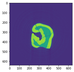
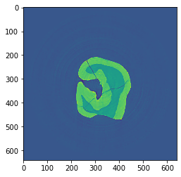
Reconstruction using FBP method with the log-polar coordinates.
[4]:
recon = tomopy.recon(proj,
                     theta,
                     center=rot_center,
                     algorithm=tomopy.lprec,
                     lpmethod='fbp',
                     filter_name='parzen')
recon = tomopy.circ_mask(recon, axis=0, ratio=0.95)
plt.imshow(recon[0, :, :])
plt.show()
Reconstructing 48 slice groups with 2 master threads...
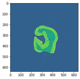
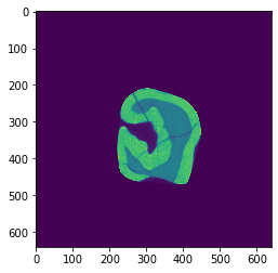
Reconstruction using the gradient descent method with the log-polar coordinates.
[5]:
recon = tomopy.recon(proj,
                     theta,
                     center=rot_center,
                     algorithm=tomopy.lprec,
                     lpmethod='grad',
                     ncore=1,
                     num_iter=64,
                     reg_par=-1)
recon = tomopy.circ_mask(recon, axis=0, ratio=0.95)
plt.imshow(recon[0, :, :])
plt.show()
Reconstructing 1 slice groups with 1 master threads...
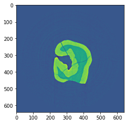
Reconstruction using the conjugate gradient method with the log-polar coordinates.
[6]:
recon = tomopy.recon(proj,
                     theta,
                     center=rot_center,
                     algorithm=tomopy.lprec,
                     lpmethod='cg',
                     ncore=1,
                     num_iter=16,
                     reg_par=-1)
recon = tomopy.circ_mask(recon, axis=0, ratio=0.95)
plt.imshow(recon[0, :, :])
plt.show()
Reconstructing 1 slice groups with 1 master threads...
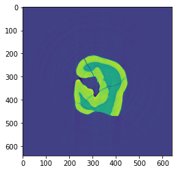
Reconstruction using the TV method with the log-polar coordinates. It gives piecewise constant reconstructions and can be used for denoising.
[7]:
recon = tomopy.recon(proj,
                     theta,
                     center=rot_center,
                     algorithm=tomopy.lprec,
                     lpmethod='tv',
                     ncore=1,
                     num_iter=512,
                     reg_par=5e-4)
recon = tomopy.circ_mask(recon, axis=0, ratio=0.95)
plt.imshow(recon[0, :, :])
plt.show()
Reconstructing 1 slice groups with 1 master threads...
Reconstruction using the TV-entropy method with the log-polar coordinates. It can be used for suppressing Poisson noise.
[8]:
recon = tomopy.recon(proj,
                     theta,
                     center=rot_center,
                     algorithm=tomopy.lprec,
                     lpmethod='tve',
                     ncore=1,
                     num_iter=512,
                     reg_par=2e-4)
recon = tomopy.circ_mask(recon, axis=0, ratio=0.95)
plt.imshow(recon[0, :, :])
plt.show()
Reconstructing 1 slice groups with 1 master threads...

Reconstruction using the TV-l1 method with the log-polar coordinates. It can be used to remove structures of an image of a certain scale, and the regularization parameter \(\lambda\) can be used for scale selection.
[9]:
recon = tomopy.recon(proj,
                     theta,
                     center=rot_center,
                     algorithm=tomopy.lprec,
                     lpmethod='tvl1',
                     ncore=1,
                     num_iter=512,
                     reg_par=3e-2)
recon = tomopy.circ_mask(recon, axis=0, ratio=0.95)
plt.imshow(recon[0, :, :])
plt.show()
Reconstructing 1 slice groups with 1 master threads...
Reconstruction using the MLEM method with the log-polar coordinates.
[10]:
recon = tomopy.recon(proj,
                     theta,
                     center=rot_center,
                     algorithm=tomopy.lprec,
                     lpmethod='em',
                     ncore=1,
                     num_iter=64,
                     reg_par=0.05)
recon = tomopy.circ_mask(recon, axis=0, ratio=0.95)
plt.imshow(recon[0, :, :])
plt.show()
Reconstructing 1 slice groups with 1 master threads...
[ ]: