Using the ASTRA toolbox through TomoPy
Here is an example on how to use the ASTRA toolbox through its integration with TomoPy, as published in [Pelt:16a].
%pylab inline
Install the ASTRA toolbox and TomoPy then:
import tomopy
DXchange is installed with tomopy to provide support for tomographic data loading. Various data format from all major synchrotron facilities are supported.
import dxchange
matplotlib provide plotting of the result in this notebook. Paraview or other tools are available for more sophisticated 3D rendering.
import matplotlib.pyplot as plt
Set the path to the micro-CT data to reconstruct.
fname = '../../tomopy/data/tooth.h5'
Select the sinogram range to reconstruct.
start = 0
end = 2
This data set file format follows the APS beamline 2-BM and 32-ID definition. Other file format readers are available at DXchange.
proj, flat, dark, theta = dxchange.read_aps_32id(fname, sino=(start, end))
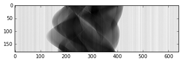
Plot the sinogram:
plt.imshow(proj[:, 0, :], cmap='Greys_r')
plt.show()
If the angular information is not avaialable from the raw data you need to set the data collection angles. In this case theta is set as equally spaced between 0-180 degrees.
if (theta is None):
    theta = tomopy.angles(proj.shape[0])
else:
    pass
Perform the flat-field correction of raw data:
proj = tomopy.normalize(proj, flat, dark)
Tomopy provides various methods to find rotation center.
rot_center = tomopy.find_center(proj, theta, init=290, ind=0, tol=0.5)
Calculate
proj = tomopy.minus_log(proj)
Reconstruction with TomoPy
Reconstruction can be performed using either TomoPy’s algorithms, or the algorithms of the ASTRA toolbox.
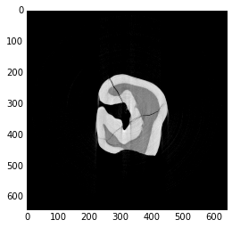
To compare, we first show how to reconstruct an image using TomoPy’s Gridrec algorithm:
recon = tomopy.recon(proj, theta, center=rot_center, algorithm='gridrec')
Mask each reconstructed slice with a circle.
recon = tomopy.circ_mask(recon, axis=0, ratio=0.95)
plt.imshow(recon[0, :,:], cmap='Greys_r')
plt.show()
Reconstruction with the ASTRA toolbox
To reconstruct the image with the ASTRA toolbox instead of TomoPy,
change the algorithm keyword to tomopy.astra, and specify the
projection kernel to use (proj_type) and which ASTRA algorithm to
reconstruct with (method) in the options keyword.
More information about the projection kernels and algorithms that are supported by the ASTRA toolbox can be found in the documentation: projection kernels and algorithms. Note that only the 2D (i.e. slice-based) algorithms are supported when reconstructing through TomoPy.
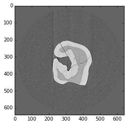
For example, to use a line-based CPU kernel and the FBP method, use:
options = {'proj_type':'linear', 'method':'FBP'}
recon = tomopy.recon(proj, theta, center=rot_center, algorithm=tomopy.astra, options=options)
recon = tomopy.circ_mask(recon, axis=0, ratio=0.95)
plt.imshow(recon[0, :,:], cmap='Greys_r')
plt.show()
If you have a CUDA-capable NVIDIA GPU, reconstruction times can be greatly reduced by using GPU-based algorithms of the ASTRA toolbox, especially for iterative reconstruction methods.
To use the GPU, change the proj_type option to 'cuda', and use
CUDA-specific algorithms (e.g. 'FBP_CUDA' for FBP):
options = {'proj_type':'cuda', 'method':'FBP_CUDA'}
recon = tomopy.recon(proj, theta, center=rot_center, algorithm=tomopy.astra, options=options)
recon = tomopy.circ_mask(recon, axis=0, ratio=0.95)
plt.imshow(recon[0, :,:], cmap='Greys_r')
plt.show()

Many algorithms of the ASTRA toolbox support additional options, which
can be found in the
documentation.
These options can be specified using the extra_options keyword.
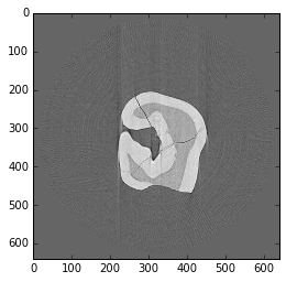
For example, to use the GPU-based iterative SIRT method with a nonnegativity constraint, use:
extra_options ={'MinConstraint':0}
options = {'proj_type':'cuda', 'method':'SIRT_CUDA', 'num_iter':200, 'extra_options':extra_options}
recon = tomopy.recon(proj, theta, center=rot_center, algorithm=tomopy.astra, options=options)
recon = tomopy.circ_mask(recon, axis=0, ratio=0.95)
plt.imshow(recon[0, :,:], cmap='Greys_r')
plt.show()